DeepRepViz - Deep Representation visualizer

DeepRepViz is an interactive web tool that can be used to inspect the 3D representations learned by predictive deep learning (DL) models. It can be used to inspect a trained model for any biases in the training and the data and debug the model. The tool is intended to help improve the transparency of such DL models. The DL models can be a ‘black box’ and hinder their adaptation to critical decision processes (ex: medical diagnosis). This tool aims to provide a platform that developers of DL models can use to gain a better intuition about what their model is learning by visualizing its ‘learned representation’^[1] of the data. It can be used to understand what the model might be basing its decisions upon.

With DeepRepViz, one can ask questions such as:

1. Debugging biases:
   
   • Is the model learning biased by demographic factors such as the sex of the subjects, their age, or their ethnicity?
     
   • Is it confounded by some spurious variable such as watermarks in the input images that accidentally correlate with the predicted label, or the type of scanner machine that is used to collect the MRIs?
2. Inspecting model learning:
   
   • Which data points is the model most confident upon? What are the characteristics of these data points? Is there some common trait among the data points that the model always misclassifies?
     
   • What variables does the model seem to capture from the data when making its predictions? For instance, consider a DL model that is used to predict fluid intelligence from brain MRI. Does the learned representation space seem to simply capture the education level of the subjects or their socio-economic status?
     
3. Debugging model training:
   
   • Is there a co-variate shift between the training data and the test data?
     

Developers can also share their model’s learned representation and the list of suspicious risk variables^[2] that can be then independently inspected and verified by other stakeholders and users of the model.

As an example, consider the below (demonstrative) scenario:

Scenario #1
Say, you developed a DL model that can diagnose Alzheimer’s disease from brain MRI with an accuracy of 80% on your test data. However, when a clinician tests your model in their hospital they complain that it is inaccurate and doesn’t perform better than chance (50%). Now you suspect that something must have gone wrong in your DL model training process or in the data used to train the model that made it incapable of generalizing to the subjects in the hospital. Either your model learned to predict Alzeihmers using some spurious shortcuts. Maybe the age of the subjects correlated with the label such that the healthy controls in your data were always younger than Alzheimer’s subjects. Or the MRI scanner machines used were different for Alzheimer’s patients and healthy controls as they were scanned at different locations. Or there is a complex spurious interaction effect in the data (as happens to be in reality) such that older subjects and subjects scanned on scanner A by chance seemed to 4 times more likely to be Alzheimer’s patients and your DL model just picked up on this relation to get 80% accuracy.

To verify, you prepare a list of ‘suspicious’ variables from your dataset, extract your model’s learned representation, upload it on DeepRepViz and inspect them (as shown in section How does DeepRepViz work?.

After testing all your suspicious variables you find that the variable age X scanner indeed shows a significantly high ‘confounding risk score’. You retrain your model by resampling the data such that this spurious relation between the age X scanner and the diagnosis label is removed. When you test the new model’s representation on the tool you see that none of the suspicious variables, including age X scanner have a high confounding risk score anymore.

How does DeepRepViz work?

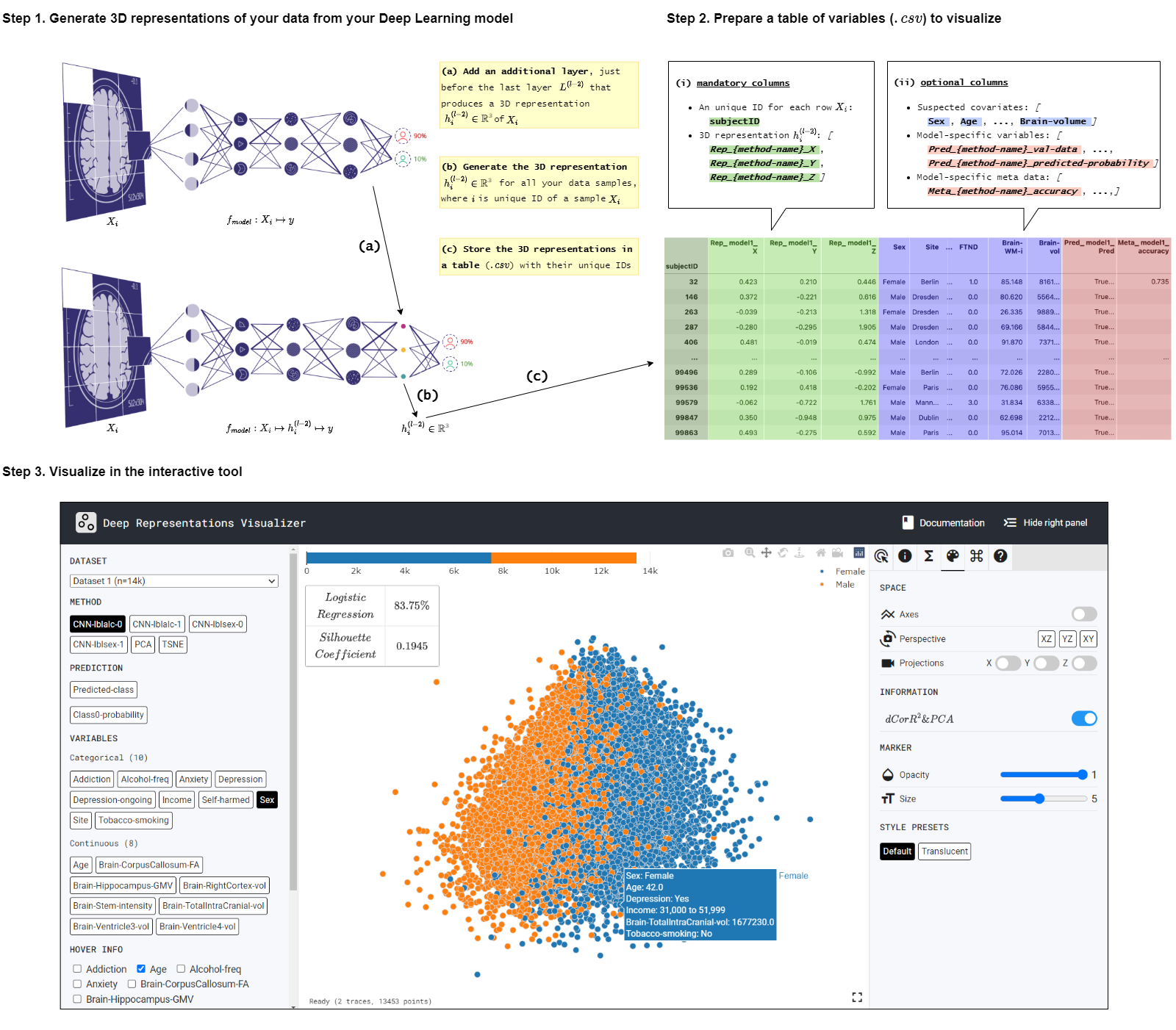
Consider a DL model f_model : X ↦ y with with l layers {L⁽⁰⁾, L⁽¹⁾, ....L^(l−2), L^(l−1)}. To inspect this model using DeepRepViz the next 3 steps can be followed (An intuitive illustration of the procedure is provided below):

Step 1. Generate 3D representation of your data from your Deep Learning (DL) model

Detail information
Add an fully-connected layer with 3 weights and no bias parameter, just before the final layer such that f_model : X ↦ h^(l−2) ↦ y where h^(l−2) ∈ ℝ³ and the model has l layers. This layer forces the DL model to learn an intermediary 3-dimensional (3D) representation that we can visualize and inspect in the DeepRepViz tool.
To save this 3D representation:
• Train the model f_model : X ↦ h^(l−2) ↦ y on the data as planned.
• Perform inference on all data points X_i  ∀i ∈ {0..N − 1} using f_model, where N is the total number of data points in the analysis. Store the intermediary representation h_i^(l−2)  ∀i ∈ {0..N − 1} generated by the model, along with the data point’s unique ID.

Step 2. Prepare a table of variables (.csv) to visualize

Detail information

The csv file uploaded on the tool will work only if it contains the below columns and column name formating:


1. subjectID (N=1): Unique IDs for each row. Acts as an index for the table. It can be any user-defined unique name used to identify a specific model and prediction task it performs. As an example, if users are trained a Convolutional Neural Network (CNN) model to predict their age from brain MRI then the columns can be named as [Rep_CNN-brainage_X], [Rep_CNN-brainage_Y], and [Rep_CNN-brainage_Z].
2. [Rep_[method name]_X, Rep_[method name]_Y, Rep_[method name]_Z] (N=1 x 3): The [X,Y,Z] coordinates of the generated 3D representation space h_i^(l−2)  ∀i ∈ {0..N − 1}. These coordinates determine the position of each subject along with a unique ID subjectID in the 3D space of the viz tool.
3. [variable name](optional) (N=inf): These are the variables whose distribution you wish to visualize with respect to the 3D representation space. When this variable is selected on the tool, each subject is colored by the value of this variable. Append all potential confounding variables to the table as additional columns. Variables with numerical values will be interpreted by the tool as an ordinal or an interval type and variables with string values will be interpreted as nominal type. However, this can be interchanged later in the tool. There is no limit to how many variables are added. In the above example these are the variables age, sex, FTND, total brain volume, ventricles size and hippocampus area. Can be continuous or categorical.
4. Pred_[method name]_[pred info name] (optional) (N=inf): You can provide method-specific information for each method about the each subject. Can be continuous or categorical. Ex: for methods using machine learning / deep learning models, you can provide which subjects were predicted correctly, which subjects were used as the test subjects, what was the probability of model prediction for each subject.
5. Meta_[method name]_[meta info name] (optional) (N=inf): You can provide method-specific meta data information that you want to show in the tool in general. Ex: for methods using machine learning / deep learning models, you can provide the prediction accuracy of that model and information about the model architecture. Ex2: for PCA method you can provide the % of explained variance by [X,Y,Z].
   
   

   (Note 1: text under [] such as [method name] and [variable name] means it can be anything the user chooses and it will be displayed by that name in the tool)
   (Note 2: When the columns marked as (optional) are not included in the csv, the tool will still work.)
   (Note 3: (N=i) indicates how many of these column instances are expected. (N=inf) implies that there is no limit to the number of these columns)
   

Step 3. Visualize on the interactive tool

Detail information

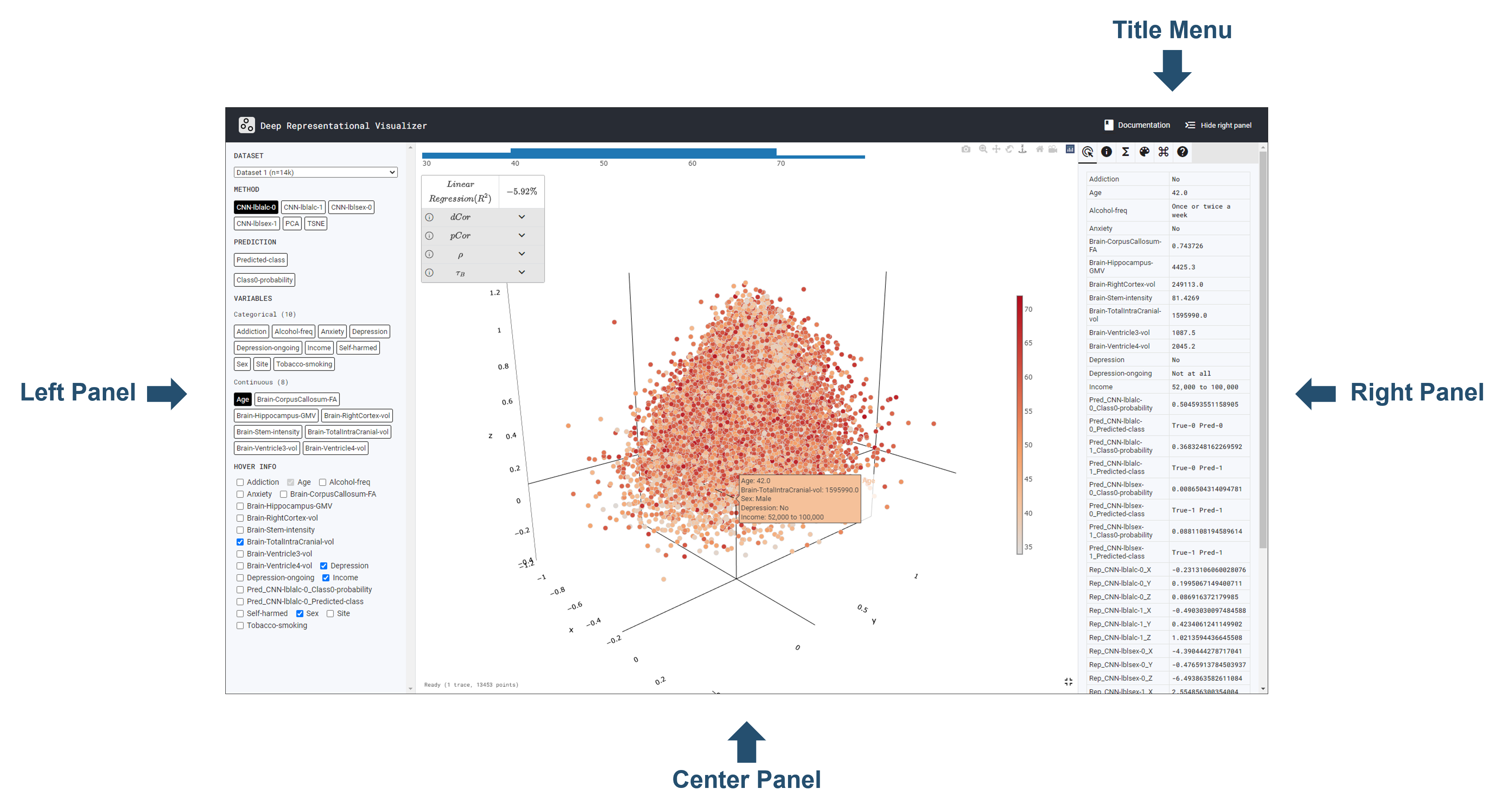
The learned representation space of the DL model is displayed at the center. Users can interactively inspect this representation space using various features available in the panel on the right. From the panel on the left, users can select different ‘potential confound’ variables and color-code the representation space in the center. The tool also computes the confounding risk scores for the selected variable as shown in the top left corner of the central display. Find out more in the next section Graphic User Interface (GUI) Features.

Graphic User Interface (GUI) Features

A brief demonstration

Let’s take a closer look at the components of the DeepRepViz interface:

Title Menu

Detail information

Documentation hyperlink to the DeepRepViz documentation, and Hide Right Panel, this function hides the right panel.

Left Panel

Detail information
The left panel has four areas; Dataset, Method, Colum, and Hover Info from top to bottom.

1. In , by defualt, Dataset 1 (n=14k) is selected. You can also select another dataset or upload your own dataset, which is prepared by Step 2. Prepare a table of variables (.csv) to visualize.
   
2. In , you can check the available METHOD(s).
   
3. In , you can explore the options; prediction labels, categorical variables, and continuous variables. explain which prediction it is. You can also select different ‘potential confound’ variables with only one selection either or .
   
4. In , you can select multiple hover info, which display on the center panel.

Center Panel

Detail information
Top Button
1. In , you can check the range of the dataset, and filter the range only if continuous variables in the top left corner of the central panel.
2. In the below filter, , the tool also dispaly the confounding risk scores for the selected variable.
3. In , you can use the plotly modebar function as shown in the top right corner. More detail can be found in An Introduction to Chart Studio Modebar.
4. By clicking the variable name; , in the blow plotly, you can explore the dataset representation within the desired categorical variable within the dataset.
Main Windows
The learned representation space of the DL model is displayed at the center. Color-code the representation space in the center.
Bottom Button
On the right bottom, Full Screen supports full screen function.

Right Panel

Detail information
The 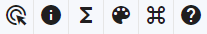Settings Bar under the Title Menu supports the following functions for representation space:


1. Datapoint represent each columns information.
2. Metadata only if shows the model’s metadata; for examples, please check the dataset 2 case.
3. Transform can do such as Min-Max Scaling, Standardization, PCA and displayed ALL Stats.
4. With Styling users can do such space, infromation, and maerker change. It also provided style presets.
5. On Shortcuts, it provides how to use the shorcuts key.
6. About shows the App version.

Two demonstrative examples:

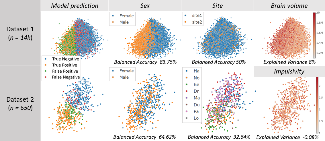
In the below examples, inspecting two predictive DL models using DeepRepViz helped us find spurious confounder variables and biases in the models:

Dataset 1

We predicted alcohol drinking frequency from brain MRI. Model prediction boundary aligns with Sex and Brain volume of the subjects, but not with the Site variable. The confounding risk scores also reflects this. This suggests that the DL model may have simply predicted all males in the data and subjects with large brain volume as frequent drinkers.


Dataset 2

We predict a social behavior (detail held for anonymity) from brain MRI. Here the Site variable seems to confound the model predictions. It can be observed, for instance, that all subjects from the Dr site (see legend of Site) are categorized by the model as having risky category of the social behavior, whereas all subjects from the No site are exclusively predicted as have a safe social behavior. To prevent this spurious effect, the MRI dataset can be harmonized across the different sites where the data was collected.

Acknowlegement

This project was inspired by Google Brain’s projector.tensorflow.org, but is more catering towards the medical domain and medical imaging analysis. For implementation, we heavily rely on 3D-scatter-plot from plotly.js.

Citations

[1] Bengio, Yoshua, Aaron Courville, and Pascal Vincent. “Representation learning: A review and new perspectives.” IEEE transactions on pattern analysis and machine intelligence 35.8 (2013): 1798-1828.
[2] Görgen, Kai, et al. “The same analysis approach: Practical protection against the pitfalls of novel neuroimaging analysis methods.” Neuroimage 180 (2018): 19-30.

Last updated 2022-10-24 UTC.